Google Sheets - Alternating Colors
One popular request I often get from people that are looking at large sheets with lots of data is how to alternate the color of the rows to make it easier to read across and not lose your line. Setting alternating colors is very easy with Google Sheets. Simply -
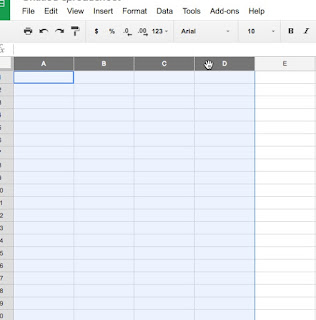
1. Highlight the columns you want to assign alternating colors to
2. Go to the Format Menu and select Alternating colors... (towards the bottom of the menu)
3. Set your formatting -
A. Choose if you have a header and/or footer on your sheet - it will use darker highlights on those cells
B. Select the Formatting styles that are preset OR click on the + to create a custom style
C. Make any modifications you would like to the colors (Note: if you selected a preset style, as soon as you make a color change it will create a custom style)
6. Click Done
If you want to remove alternating colors, go back to the Format Menu and select Alternating colors... and at the bottom of the window is the choice "Remove alternating colors."
1. Highlight the columns you want to assign alternating colors to
2. Go to the Format Menu and select Alternating colors... (towards the bottom of the menu)
A. Choose if you have a header and/or footer on your sheet - it will use darker highlights on those cells
B. Select the Formatting styles that are preset OR click on the + to create a custom style
C. Make any modifications you would like to the colors (Note: if you selected a preset style, as soon as you make a color change it will create a custom style)
6. Click Done
If you want to remove alternating colors, go back to the Format Menu and select Alternating colors... and at the bottom of the window is the choice "Remove alternating colors."


